
|
AISpace2 | Main Tools | News | Downloads | Prototype Tools | Customizable Applets | Practice Exercises | Help | About AIspace |
|
|
Tutorials
Decision Trees
Tutorial 2: Building a Decision TreeOnce you have created or acquired a dataset and distributed examples between the test and training sets (using the "View/Edit Examples" window), you are ready to begin building the tree. Switch to the "Solve" mode, by clicking on the tab. The decision tree is visualized as a set of nodes, edges, and edge labels. Each node in the tree represents an input parameter that examples are split on. Red rectangles represent interior nodes while green rectangles represent leaf nodes. Blue rectangle nodes are nodes that have not yet been split. The labels on the edges between nodes indicate the possible values of the parent split parameter. After acquiring a dataset and switching to Solve mode, your applet should look like this: 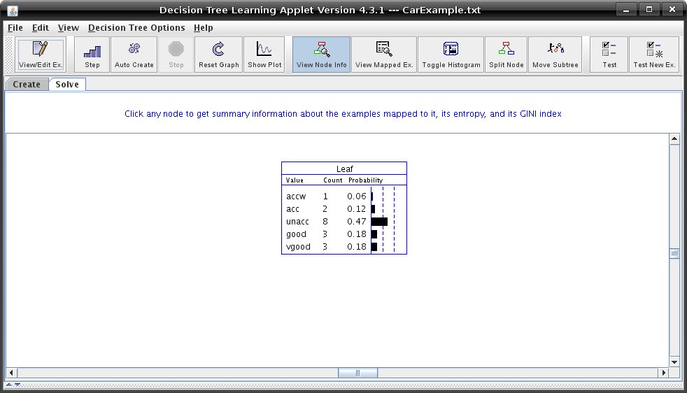 A blue node is a node that has not been split. To find a legend of the node's colours and shapes, go to the help menu and click on "Legend for nodes/edges". Before you begin building your tree, first select the splitting function to use from the "Decision Tree Options" menu. This splitting function will determine how the program chooses a parameter to split examples on. You can choose Random, Information Gain, Gain Ratio, or GINI. See Tutorial 4 on splitting algorithms to find out more information about these algorithms. There are two ways to construct a decision tree. Constructing a Tree ManuallyYou can also construct a tree by selecting parameters to split on yourself. When the node options is set to "Split Node," you can click on any blue node to split it. You can change what kind of information is displayed when clicking on a node, by changing the node's modes. The buttons that change the node's modes are the "View Node Info", "View Mapped Examples", "Toggle Histogram" and "Split Node". If you click on a node in "Split Node" mode, a window like the one below will appear with information about each of the parameters that the examples can be split on. When you have chosen a parameter, select its checkbox and click "Split." 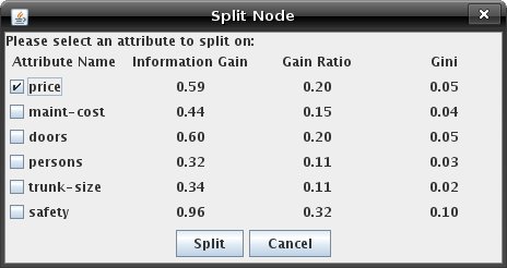 Constructing a Tree AutomaticallyAfter selecting a splitting function, simply click "Step" to watch the program construct the tree. Clicking "Auto Create" will cause the program to continue stepping until the tree is complete or the "Stop" button is pressed. Conditions can be used to restrict splitting while automatically generating a tree. To set stopping conditions, click "Stopping Conditions..." from the "Decision Tree Options" menu. Clicking the checkbox beside a condition enables it and allows you to edit the parameter that appears to the right of the condition. The program will not split a node if any enabled stopping condition is met. Below is an example of "Stopping Conditions..." dialog. 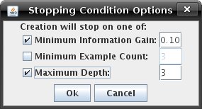 - The minimum information gain condition will prevent splits that do not produce the information gain specified by the parameter. - The minimum example count condition will not allow a node to be split if there are fewer than the specified number of examples mapped to it. - The maximum depth condition will restrict splits if they will increase the maximum root-to-leaf depth of the tree beyond the specified value. Note that the root has depth 0. Press "Auto Create" to build the rest of your decision tree. Once it is
finished it will look similar to the one below. 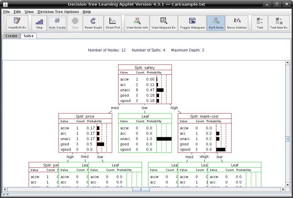 Several tools are available to guide your splitting choices: When the "View Node Information" is selected, you can click any node to get summary information about the examples mapped to it, its entropy, and its GINI index: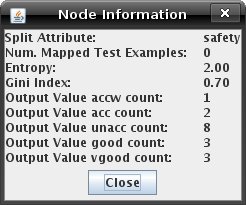 Clicking a node in "View Mapped Examples" mode will show you the examples that have been mapped to the node: 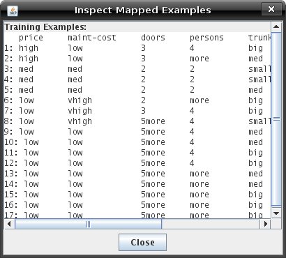 "Toggle Histogram" mode allows you to quickly enable/disable a node's histogram (which shows the output value probability distribution of the node). "Show Plot" button on the toolbar opens a plot of training and test set error over the number of splits. This can be useful for evaluating whether or not further splitting is likely to improve the decision tree's predictions. The type of error plotted can be changed via the tabs on the error plot window. The two error calculations are average sum of absolute values of differences between the predicted distribution and the actual distribution, and a squared variant of this, the average sum of squares of values of differences. 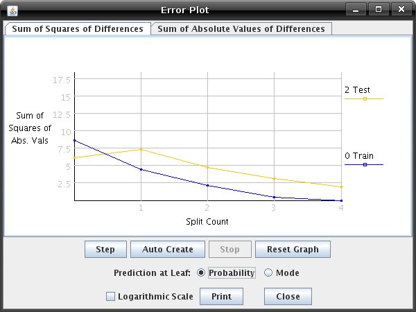
To test your decision tree see Tutorial 3. |
| Main Tools: Graph Searching | Consistency for CSP | SLS for CSP | Deduction | Belief and Decision Networks | Decision Trees | Neural Networks | STRIPS to CSP |