Back to Tutorials.

Tutorial 3: Solving a Neural Network

This tutorial will use the Mail Reading example to demonstrate the basic solving and testing of your neural network.
This tutorial will cover the rudimentary elements - after you load a pre-existing graph you can change the mode to the 'Solve' mode, in which you can solve the graph.
Click on Initialize Parameters to reset the learning of your network. By default, Initialize Parameters will assign random values in the range [-1,1] to parameters. This option can be modified by clicking on 'Parameter Initialization Options...' under the Neural Options menu. Your graph should now look like this:

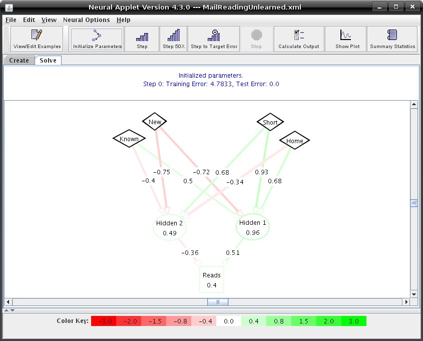When you initialize the parameters, the nodes and edges may change colors corresponding to their values. In the 'Help' menu you can click on 'Legend for Nodes/Edges' to make the legend below appear.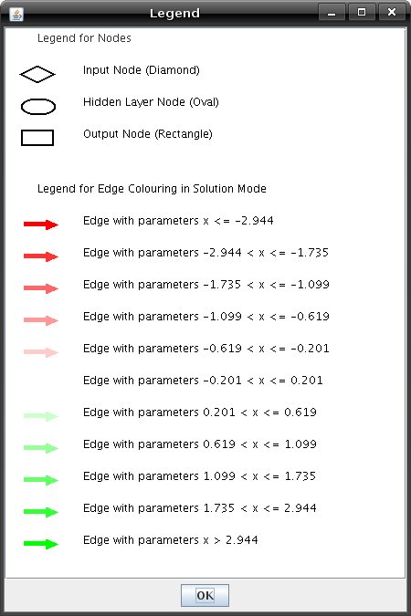

If you would like to modify your network, click on the tab marked 'Create' to return to create mode.

There are three ways to perform backpropagation in the Neural Networks applet.

1. Step through the process one step at a time by clicking the Step button.

2. Step through the process 50 steps at a time by clicking the Step 50X button.

3. Allow the applet to solve to a preset minimum error (.1 by default) by clicking the Step To Target Error button.

When performing multiple steps, you can stop stepping by clicking the Stop button

Feedback

The message at the top of the network canvas will tell you how many steps you have currently run and what the error is for the training examples and the test examples, so you can decide to do more stepping or not. Below is an example of the message panel: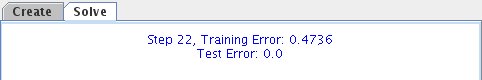

To show the error plot, click the Show Plot button.

The error values of the training and the test sets are displayed on the right side of the plot. The blue plot is the training set error, while the orange plot is the test set error. The plot window shows a graph of the error of the neural network. As the backpropagation algorithm is run, the error should be minimized.

The plot window also has Initialize Parameters, Step, Step X, Step to Target Error, and Stop buttons, which work in the same way as their solve mode counterparts. In addition, there are buttons to close, clear, and print the plot window. There is also a checkbox to switch between logarithmic and standard display modes. Below is an example of what your error plot may look like: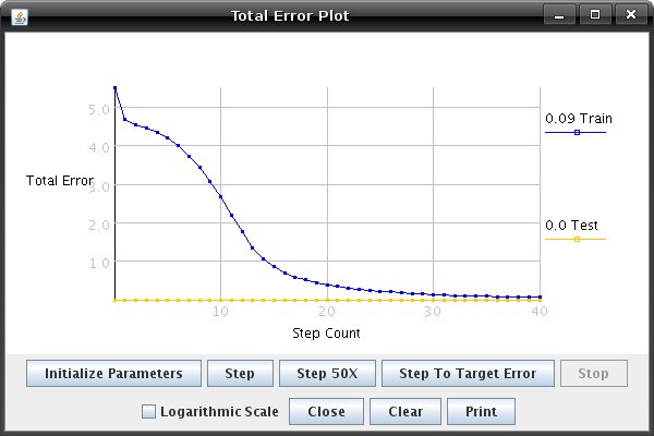

To get an output given a set of inputs, click the Calculate Output button and enter the desired inputs. The inputs given are NOT added to the test or training sets. Also, these inputs do not affect the learning of the network in any way. Below is an example of what your output dialog box will look like: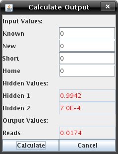

The Summary Statistics Window displays statistics for the test set, and as such, can only be pulled up once there is at least one example in the test set. The window displays all the test examples as a table, as well as the predicted value. It classifies the examples as correct or incorrect depending on a classification range which is determined by the user. This "threshold" defaults to .5. The window also gives a percentage correct or incorrect, and also allows the user to select which output's predicted value is displayed in the table.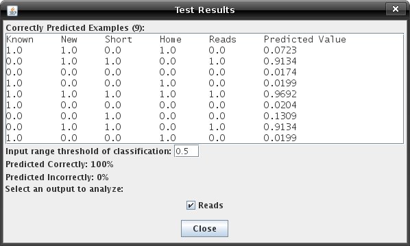

To learn how to use the view/edit examples refer to Tutorial 1.